In this article, I will show step by step how you can apply conditional formatting to multiple cells. As an example, I am going to take a small set of hypothetical data and apply conditional formatting to the background color of these cells per the value of the temperature data they contain. Let’s use blue to represent cold temperatures less than 10 degrees, green color to represent pleasant temperature 11 to 25 degrees, and red to represent hot temperatures more than 25 degrees. Let’s get started:
Using conditional formatting in Google Sheets
Step 1: Visit Google Sheets and start a blank sheet. Step 2: Prepare two columns “Days” and “Temperature” in D and E respectively as shown in the reference figure.
Step 3: Let’s assume that temperature below 10C is the coldest on our scale and we want to color the background of the cell dark blue when the temperature is below 10C. Step 4: For the case in the previous step let’s add a rule in cell E10. Click on the “Format” menu and then on “Conditional formatting”. A small “Conditional formatting” window will appear to the right of the screen.
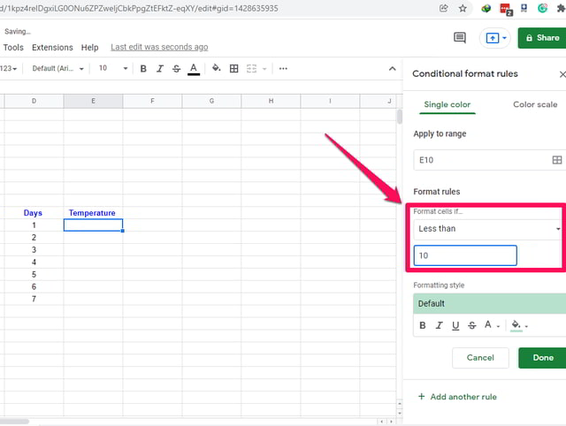
Step 5: In this window in the “Format rules” section click on the “Is not empty” box to get a drop-down menu. Scroll down and find the option “Less than” and select it by clicking on it.
Step 6: In the “value or formula box” enter the value 10. Step 7: In the “Format style” section click on the button with the half-filled bucket icon. A color options window will appear. In this window select the dark blue color.
Step 8: Next to add the case of pleasant temperature click on the “+ Add another rule” at the bottom of the window.
Step 9: This time in the “Format rules” section choose the “Is between” option and type 10 and 25 in the empty boxes respectively. Step 10: In the “Formatting style” section choose the green color. Then click on the “+ Add another rule” to add the last rule.
Step 11: For the last case in the “Format rules” section choose the “Greater than” option and type 25 in the empty box after it.
Step 12: In the “Formatting style” section choose the red color and then click on the green “Done” button. The three rules have been added. Next is to extend the formatting to multiple cells and then add some sample data to see the behavior. Step 13: Point your cursor to the small blue square in the cell highlighter in cell E10. The cursor will change to a bigger plus icon.
Step 14: Press the left mouse button and while keeping it pressed, scroll down to copy and paste the formatting of cell E10 to the cells below it. Step 15: Enter 3, 12, and 30 in the cells E10, E11, and E12 respectively. You will notice that the background of these cells has changed automatically to their configured formatting rules.
Step 16: As the last step, enter any data of your choice in the remaining cells and note its behavior.
Wrapping Up
This article showed step by step the use of conditional formatting in Google Sheets to a small set of hypothetical temperature data. Play around the conditional formatting option in Google Sheets using our example or use your own and let me know about the results in the comments section.


